
Internal linking optimization is critical if you want your site pages to have enough authority to rank for their target keywords. Internal linking refers to pages on your website that receive links from other pages.
This is significant because it is the basis for Google and other search engines determining the importance of the page concerning other pages on your website.
It also influences how likely a user is to find content on your site. The Google PageRank algorithm is based on content discovery.
Today, we’re looking into a data-driven approach to improving a website’s internal linking for better technical site SEO. That is, the distribution of internal domain authority should be optimized based on the site structure.
Read A Beginner’s Guide to Digital Marketing.
Using Data Science to Improve Internal Link Structures
Our data-driven approach will concentrate on just one aspect of optimizing internal link architecture: modeling the distribution of internal links by site depth and then targeting the pages that are lacking links for their specific site depth.
We begin by importing the libraries and data, then we clean up the column names before previewing them:
import pandas as pd
import numpy as np
site_name = 'ON24'
site_filename = 'on24'
website = 'www.on24.com'

# import Crawl Data
crawl_data = pd.read_csv('data/'+ site_filename + '_crawl.csv')
crawl_data.columns = crawl_data.columns.str.replace(' ','_')
crawl_data.columns = crawl_data.columns.str.replace('.','')
crawl_data.columns = crawl_data.columns.str.replace('(','')
crawl_data.columns = crawl_data.columns.str.replace(')','')
crawl_data.columns = map(str.lower, crawl_data.columns)
print(crawl_data.shape)
print(crawl_data.dtypes)
Crawl_data

(8611, 104)

url                          object
base_url                     object
crawl_depth                  object
crawl_status                 object
host                         object
                             ...
redirect_type                object
redirect_url                 object
redirect_url_status          object
redirect_url_status_code     object
unnamed:_103                float64
Length: 104, dtype: object
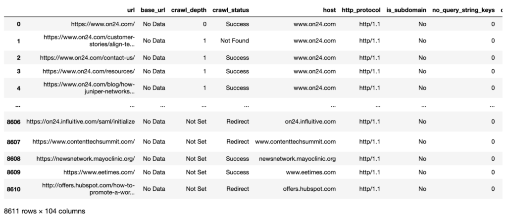
The data imported from the Sitebulb desktop crawler application is shown above as a preview. There are over 8,000 rows, and not all of them will be unique to the domain, as resource URLs and external outbound link URLs will be included.
We also have over 100 columns that aren’t required, so some column selection will be necessary.
But, before we get there, let’s take a look at how many site levels there are:
crawl_depth
0             1
1            70
10            5
11            1
12            1
13            2
14            1
2           303
3           378
4           347
5           253
6           194
7            96
8            33
9            19
Not Set    2351
dtype: int64
So, as we can see from the above, there are 14 site levels, the majority of which are found in the XML sitemap rather than the site architecture.
You’ll notice that Pandas (the Python data-handling package) sorts the site levels by digit.
This is because the site levels are currently charactered strings rather than numeric. This will be changed in later code because it affects data visualization (‘viz’).
We’ll now filter the rows and select the columns.
# Filter for redirected and live links
redir_live_urls = crawl_data[['url', 'crawl_depth', 'http_status_code', 'indexable_status', 'no_internal_links_to_url', 'host', 'title']]
redir_live_urls = redir_live_urls.loc[redir_live_urls.http_status_code.str.startswith(('2'), na=False)]
redir_live_urls['crawl_depth'] = redir_live_urls['crawl_depth'].astype('category')
redir_live_urls['crawl_depth'] = redir_live_urls['crawl_depth'].cat.reorder_categories(['0', '1', '2', '3', '4',
                                                                                 '5', '6', '7', '8', '9',
                                                                                        '10', '11', '12', '13', '14',
                                                                                        'Not Set',
                                                                                       ])
redir_live_urls = redir_live_urls.loc[redir_live_urls.host == website]
del redir_live_urls['host']
print(redir_live_urls.shape)
Redir_live_urls

(4055, 6)
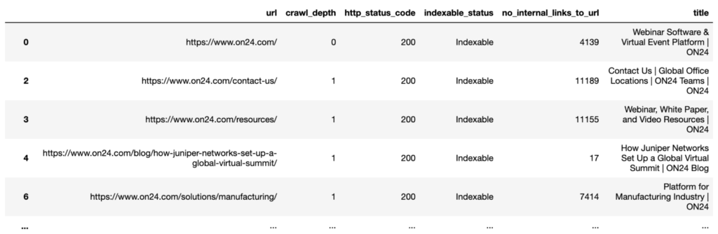
We now have a more streamlined data frame after filtering rows for indexable URLs and selecting the relevant columns (think Pandas version of a spreadsheet tab).
Investigating the Distribution of Internal Links
We’re now ready to data visualize the data and see how the internal links are distributed overall and by site depth.
from plotnine import *
import matplotlib.pyplot as plt
pd.set_option('display.max_colwidth', None)
%matplotlib inline

# Distribution of internal links to URL by site level
ove_intlink_dist_plt = (ggplot(redir_live_urls, aes(x = 'no_internal_links_to_url')) +
                    geom_histogram(fill = 'blue', alpha = 0.6, bins = 7) +
                    labs(y = '# Internal Links to URL') +
                    theme_classic() +
                    theme(legend_position = 'none')
                   )

ove_intlink_dist_plt
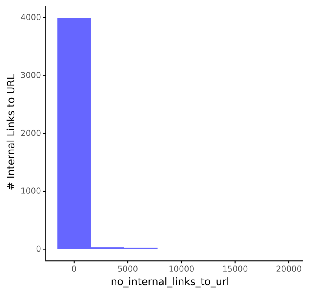
We can see from the above that most pages have no links, so improving internal linking would be a significant opportunity to improve SEO here.
Let’s look at some statistics at the site level.
crawl_depth
0             1
1            70
10            5
11            1
12            1
13            2
14            1
2           303
3           378
4           347
5           253
6           194
7            96
8            33
9            19
Not Set    2351
dtype: int64
The table above depicts the approximate distribution of internal links by site level, including the average (mean) and median values (50 percent quantile).
This is in addition to the variation within the site level (std for standard deviation), which tells us how close the pages within the site level are to the average; i.e., how consistent the internal link distribution is with the average.
Except for the home page (crawl depth 0) and the first level pages (crawl depth 1), we can deduce that the average by site-level ranges from 0 to 4 per URL.
For a more visual approach, consider:
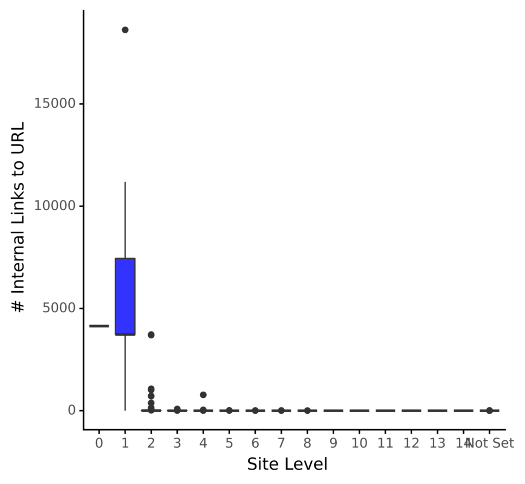
# Distribution of internal links to URL by site level
intlink_dist_plt = (ggplot(redir_live_urls, aes(x = 'crawl_depth', y = 'no_internal_links_to_url')) +
                    geom_boxplot(fill = 'blue', alpha = 0.8) +
                    labs(y = '# Internal Links to URL', x = 'Site Level') +
                    theme_classic() +
                    theme(legend_position = 'none')
                   )

intlink_dist_plt.save(filename = 'images/1_intlink_dist_plt.png', height=5, width=5, units = 'in', dpi=1000)
intlink_dist_plt
The plot above confirms our previous observations that the home page and the pages directly linked from it receive the lion’s share of the links.
With the scales as they are, we don’t have a good idea of how the lower levels are distributed. We’ll fix this by taking the y axis logarithm:
# Distribution of internal links to URL by site level
from mizani.formatters import comma_format

intlink_dist_plt = (ggplot(redir_live_urls, aes(x = 'crawl_depth', y = 'no_internal_links_to_url')) +
                    geom_boxplot(fill = 'blue', alpha = 0.8) +
                    labs(y = '# Internal Links to URL', x = 'Site Level') +
                    scale_y_log10(labels = comma_format()) +
                    theme_classic() +
                    theme(legend_position = 'none')
                   )

intlink_dist_plt.save(filename = 'images/1_log_intlink_dist_plt.png', height=5, width=5, units = 'in', dpi=1000)
intlink_dist_plt
The graph above depicts the same distribution of the links in a logarithmic view, which helps us confirm the distribution averages for the lower levels. This is much easier to picture.
The disparity between the first two site levels and the remaining site suggests a skewed distribution.
As a result, I’ll logarithmize the internal links to help normalize the distribution.
We now have the normalized number of links, which we will depict:
# Distribution of internal links to URL by site level
intlink_dist_plt = (ggplot(redir_live_urls, aes(x = 'crawl_depth', y = 'log_intlinks')) +
                    geom_boxplot(fill = 'blue', alpha = 0.8) +
                    labs(y = '# Log Internal Links to URL', x = 'Site Level') +
                    #scale_y_log10(labels = comma_format()) +
                    theme_classic() +
                    theme(legend_position = 'none')
                   )

intlink_dist_plt
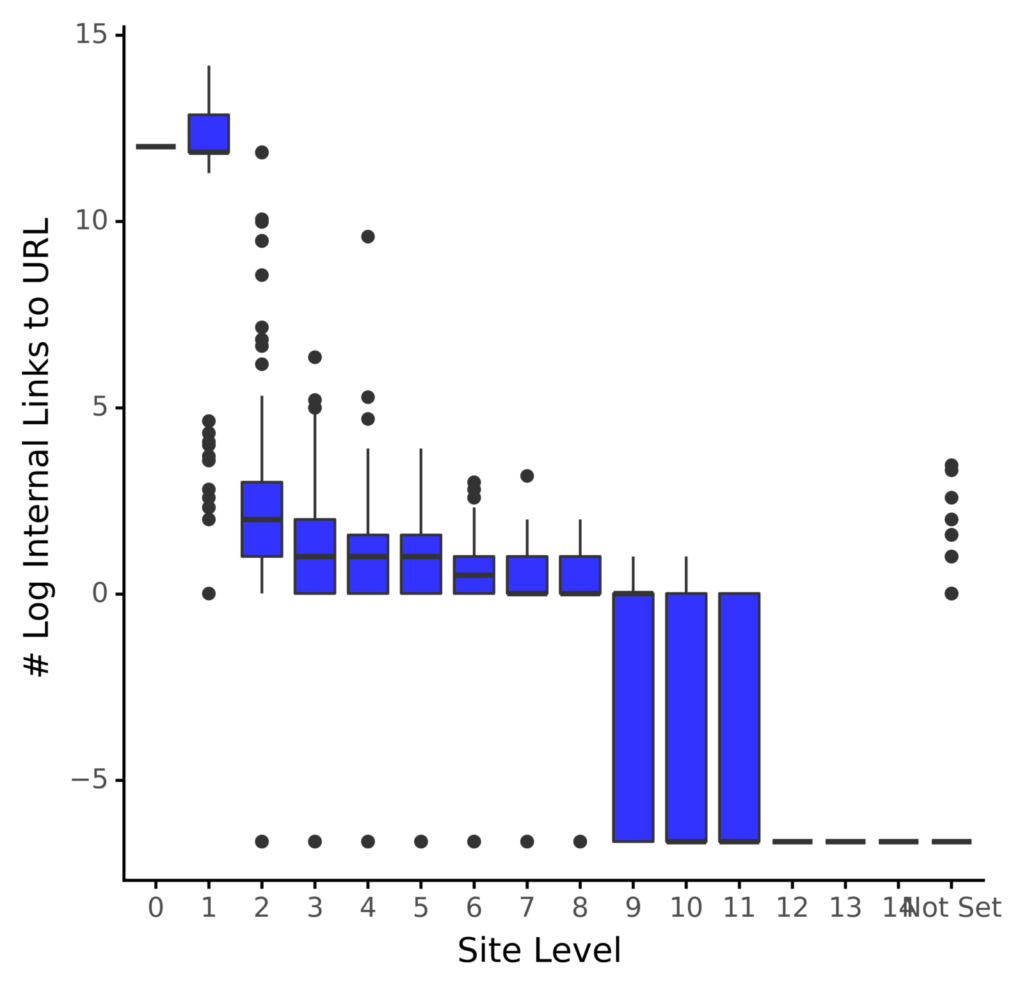
The distribution appears to be less skewed from the above, as the boxes (interquartile ranges) have a more gradual step change from site to site.
This sets us up nicely for analyzing the data and determining which URLs are under-optimized in terms of internal links.
Quantifying the Problems
For each site depth, the code below will compute the lower 35th quantile (data science term for percentile).
# internal links in under/over indexing at site level
# count of URLs under indexed for internal link counts

quantiled_intlinks = redir_live_urls.groupby('crawl_depth').agg({'log_intlinks':
                                                                 [quantile_lower]}).reset_index()
quantiled_intlinks = quantiled_intlinks.rename(columns = {'crawl_depth_': 'crawl_depth',
                                                          'log_intlinks_quantile_lower': 'sd_intlink_lowqua'})
quantiled_intlinks
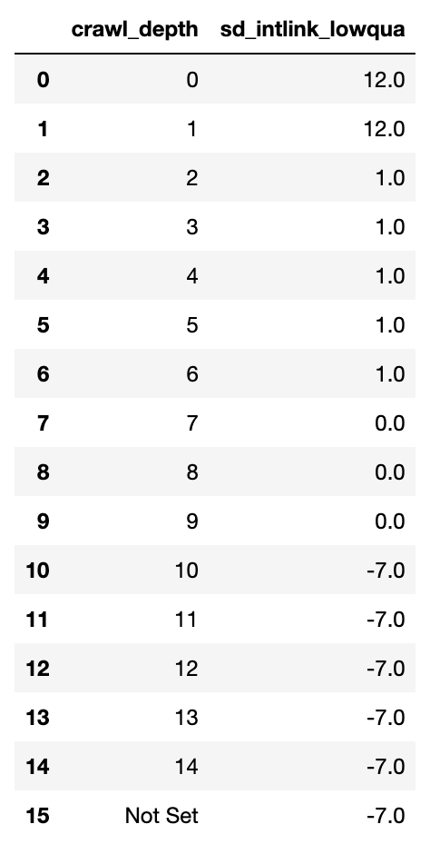
The calculations are shown above. At this point, the numbers are meaningless to an SEO practitioner because they are arbitrary and serve only to provide a cut-off for under-linked URLs at each site level.
Now that we have the table, we’ll combine it with the main data set to determine whether the URL is under-linked row by row.
# join quantiles to main df and then count
redir_live_urls_underidx = redir_live_urls.merge(quantiled_intlinks, on = 'crawl_depth', how = 'left')

redir_live_urls_underidx['sd_int_uidx'] = redir_live_urls_underidx.apply(sd_intlinkscount_underover, axis=1)
redir_live_urls_underidx['sd_int_uidx'] = np.where(redir_live_urls_underidx['crawl_depth'] == 'Not Set', 1,
                                                   redir_live_urls_underidx['sd_int_uidx'])

redir_live_urls_underidx
We now have a data frame with each URL marked as under-linked as a 1 in the “sd int uidx’ column.
This allows us to calculate the number of under-linked site pages by site depth:
# Summarise int_udx by site level
intlinks_agged = redir_live_urls_underidx.groupby('crawl_depth').agg({'sd_int_uidx': ['sum', 'count']}).reset_index()
intlinks_agged = intlinks_agged.rename(columns = {'crawl_depth_': 'crawl_depth'})
intlinks_agged['sd_uidx_prop'] = intlinks_agged.sd_int_uidx_sum / intlinks_agged.sd_int_uidx_count * 100
print(intlinks_agged)
  crawl_depth  sd_int_uidx_sum  sd_int_uidx_count  sd_uidx_prop
0            0                0                  1      0.000000
1            1               41                 70     58.571429
2            2               66                303     21.782178
3            3              110                378     29.100529
4            4              109                347     31.412104
5            5               68                253     26.877470
6            6               63                194     32.474227
7            7                9                 96      9.375000
8            8                6                 33     18.181818
9            9                6                 19     31.578947
10          10                0                  5      0.000000
11          11                0                  1      0.000000
12          12                0                  1      0.000000
13          13                0                  2      0.000000
14          14                0                  1      0.000000
15     Not Set             2351               2351    100.000000
We can now see that, even though the site depth 1 page has a higher than average number of links per URL, 41 pages are under-linked.
To be more specific:
# plot the table
depth_uidx_plt = (ggplot(intlinks_agged, aes(x = 'crawl_depth', y = 'sd_int_uidx_sum')) +
                    geom_bar(stat = 'identity', fill = 'blue', alpha = 0.8) +
                    labs(y = '# Under Linked URLs', x = 'Site Level') +
                    scale_y_log10() +
                    theme_classic() +
                    theme(legend_position = 'none')
                   )

depth_uidx_plt.save(filename = 'images/1_depth_uidx_plt.png', height=5, width=5, units = 'in', dpi=1000)
depth_uidx_plt
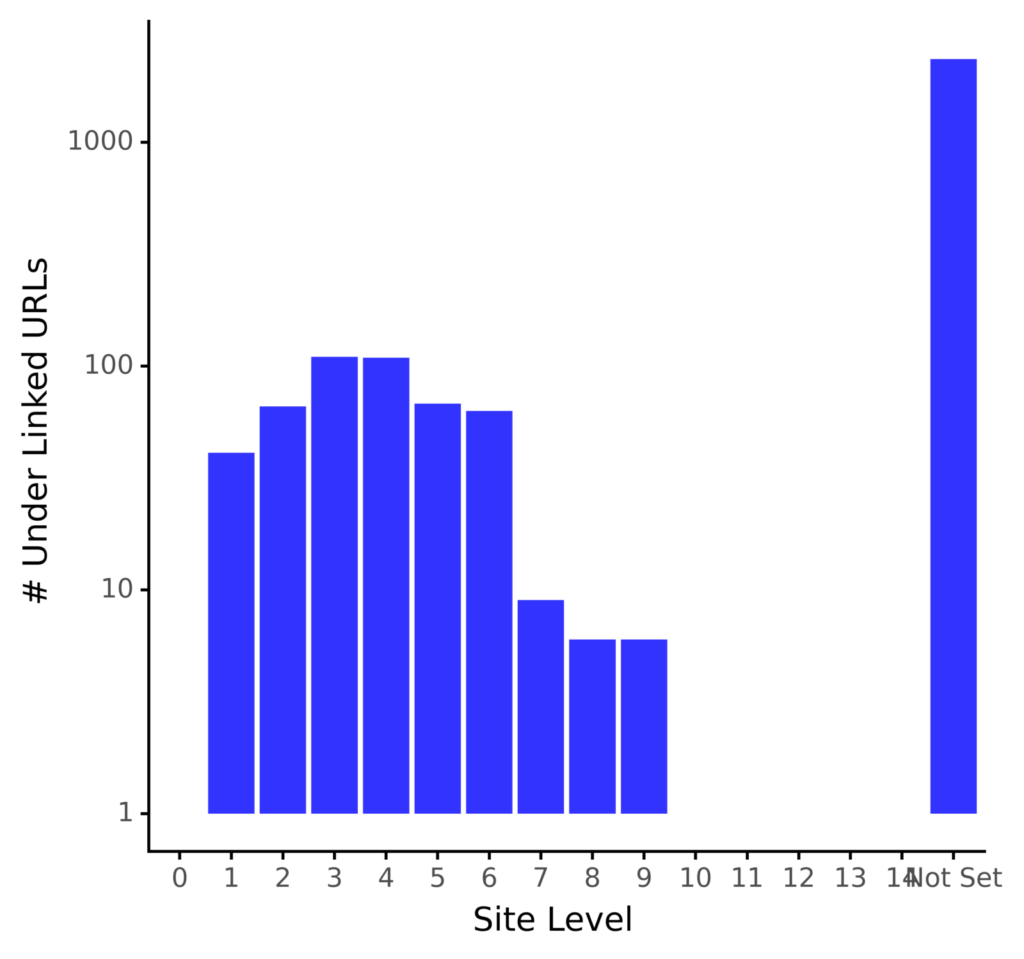
The distribution of under-linked URLs appears normal, except the XML sitemap URLs, as indicated by the near bell shape. The majority of the unlinked URLs are in site levels 3 and 4.
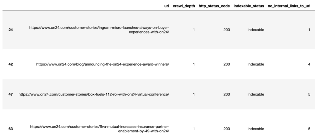
Exporting a List of Underlying URLs
Now that we’ve identified the under-linked URLs by site level, we can export the data and devise creative solutions to bridge the site depth gaps, as shown below.
# data dump of under performing backlinks
underlinked_urls = redir_live_urls_underidx.loc[redir_live_urls_underidx.sd_int_uidx == 1]
underlinked_urls = underlinked_urls.sort_values(['crawl_depth', 'no_internal_links_to_url'])
underlinked_urls.to_csv('exports/underlinked_urls.csv')
underlinked_urls
Other Internal Linking Data Science Techniques
We briefly discussed why improving a site’s internal links is important before delving into how internal links are distributed across the site by site level.
Then, before exporting the results for recommendations, we quantified the extent of the under-linking problem both numerically and visually.
Naturally, site-level internal links are only one aspect of internal links that can be statistically explored and analyzed.
Other factors that could be used to apply data science techniques to internal links include, but are not limited to:
- Page-level authority offsite.
- The importance of anchor text.
- Intention to search.
- Look for the user journey.
Need help with our free SEO tools? Try our free Plagiarism Checker, Article Rewriter, Word Counter.
Learn more from SEO and read 11 Methods for Creating a Google Algorithm Update Resistant SEO Strategy


2 Comments